3. Linear Neural Networks
Linear Regression [8]
-
MiniBatch SGD
-
matrix-derivatives
Softmax
\[\hat{\mathbf{y}} = \mathrm{softmax}(\mathbf{o})\quad \text{其中}\quad \hat{y}_j = \frac{\exp(o_j)}{\sum_k \exp(o_k)}\]Numerical stability: \(\hat{\mathbf{y}} = \mathrm{softmax}(\mathbf{o-max(o)})\quad \text{其中}\quad \hat{y}_j = \frac{\exp(o_j-max(o))}{\sum_k \exp(o_k-max(0))}\)
\[\begin{aligned} \log{(\hat y_j)} & = \log\left( \frac{\exp(o_j)}{\sum_k \exp(o_k)}\right) \\ & = \log{(\exp(o_j))}-\log{\left( \sum_k \exp(o_k) \right)} \\ & = o_j -\log{\left( \sum_k \exp(o_k) \right)}. \end{aligned}\]def softmax(X):
X_exp = torch.exp(X)
partition = X_exp.sum(1, keepdim=True)
return X_exp / partition # The broadcasting mechanism is applied here
Log-Likelihood
最大化一个似然函数同最大化它的自然对数是等价的。因为自然对数log是一个连续且在似然函数的值域内严格递增的上凹函数。注意:可能性函数(似然函数)的自然对数跟信息熵以及Fisher信息联系紧密。求对数通常能够一定程度上简化运算1

信息论的核心思想是量化数据中的信息内容,在信息论中,该数值被称为分布$P$的熵(entropy)。可以通过以下方程得到:
\[H[P] = \sum_j - P(j) \log P(j).\]当我们赋予一个事件较低的概率时,我们的惊异会更大。克劳德·香农决定用 $\log \frac{1}{P(j)} = -\log P(j)$ 来量化一个人的惊异(surprisal)。
In short, we can think of the cross-entropy classification objective in two ways:
- (i) as maximizing the likelihood of the observed data;
- (ii) as minimizing our surprisal (and thus the number of bits) required to communicate the labels.
def cross_entropy(y_hat, y):
    return -torch.log(y_hat[range(len(y_hat)), y])
5. Deep Learning Computation
CPU, GPU, TPU, FPGA, AI ASIC [31,32]
CPU: 可以处理通用计算,性能优化考虑数据读写效率和多线程
GPU: 使用更多的小核和更好的内存带宽,适合能大规模并行处理的计算任务
DSP: 数字信号处理
- 为数字信号处理算法设计:点积, 卷积, FFT
- 低功耗,高性能
- VLIW: Very Long instrction word
- 一条指令计算上百次乘累加
- 编程和调试困难
- 编译器质量良莠不齐
FPGA: 可编程阵列
- 有大量可编程逻辑单元和可配置的连接
- 可以配置成计算复杂函数
- 编程语言 VHDL, Verilog
- 比通用硬件更高效
- 编译太久
AI ASIC
- Google TPU
- 媲美Nvidia GPU
- 核心是 systolic array(大矩阵乘法) 专门为矩阵乘法定制硬件
- FPGA 可以用于验证asic设计
Transformer 适用于TPU,GPU由于内存限制,所以需要单独设计 卖芯片得有生态
Risc-V 主要是低端芯片,便宜,生态不够完善
单机多卡/分布式 [33, 34, 35]
- 数据并行
- 当数据多样性够多的情况下,大的batchsize会不收敛,因为相似的样本计算梯度意义不大
import torch

def print_fn(func):  # @save
    def wrapper(*args, **kw):
        print("[{}]:".format(func.__name__), func(*args, **kw))
    return wrapper

@print_fn
def try_gpu(i=0):  # @save
    """如果存在,则返回gpu(i),否则返回cpu()。"""
    if torch.cuda.device_count() >= i + 1:
        return torch.device(f'cuda:{i}')
    return torch.device('cpu')

@print_fn
def try_all_gpus():  # @save
    """返回所有可用的GPU,如果没有GPU,则返回[cpu(),]。"""
    devices = [torch.device(f'cuda:{i}')
               for i in range(torch.cuda.device_count())]
    return devices if devices else [torch.device('cpu')]

try_gpu()
try_gpu(10)
try_all_gpus()
[try_gpu]: cuda:0
[try_gpu]: cpu
[try_all_gpus]: [device(type='cuda', index=0), device(type='cuda', index=1), device(type='cuda', index=2), device(type='cuda', index=3), device(type='cuda', index=4), device(type='cuda', index=5), device(type='cuda', index=6), device(type='cuda', index=7)]
def train_batch_ch13(net, X, y, loss, trainer, devices):
    if isinstance(X, list):
        # 微调BERT中所需(稍后讨论)
        X = [x.to(devices[0]) for x in X]
    else:
        X = X.to(devices[0])
    y = y.to(devices[0])
    net.train()
    trainer.zero_grad()
    pred = net(X)
    l = loss(pred, y)
    l.sum().backward()
    trainer.step()
    train_loss_sum = l.sum()
    train_acc_sum = d2l.accuracy(pred, y)
    return train_loss_sum, train_acc_sum

def train_ch13(net, train_iter, test_iter, loss, trainer, num_epochs,
               devices=d2l.try_all_gpus()):
    timer, num_batches = d2l.Timer(), len(train_iter)
    animator = d2l.Animator(xlabel='epoch', xlim=[1, num_epochs], ylim=[0, 1],
                            legend=['train loss', 'train acc', 'test acc'])
    net = nn.DataParallel(net, device_ids=devices).to(devices[0])
    for epoch in range(num_epochs):
        # 4个维度:储存训练损失,训练准确度,实例数,特点数
        metric = d2l.Accumulator(4)
        for i, (features, labels) in enumerate(train_iter):
            timer.start()
            l, acc = train_batch_ch13(
                net, features, labels, loss, trainer, devices)
            metric.add(l, acc, labels.shape[0], labels.numel())
            timer.stop()
            if (i + 1) % (num_batches // 5) == 0 or i == num_batches - 1:
                animator.add(epoch + (i + 1) / num_batches,
                             (metric[0] / metric[2], metric[1] / metric[3],
                              None))
        test_acc = d2l.evaluate_accuracy_gpu(net, test_iter)
        animator.add(epoch + 1, (None, None, test_acc))
    print(f'loss {metric[0] / metric[2]:.3f}, train acc '
          f'{metric[1] / metric[3]:.3f}, test acc {test_acc:.3f}')
    print(f'{metric[2] * num_epochs / timer.sum():.1f} examples/sec on '
          f'{str(devices)}')
- 模型并行
Pytorch
MySequential
class MySequential(nn.Module):
    def __init__(self, *args):
        super().__init__()
        for block in args:
            # 这里,`block`是`Module`子类的一个实例。我们把它保存在'Module'类的成员变量
            # `_modules` 中。`block`的类型是OrderedDict。
            self._modules[block] = block

    def forward(self, X):
        # OrderedDict保证了按照成员添加的顺序遍历它们
        for block in self._modules.values():
            X = block(X)
        return X
Initialization
def init_normal(m):
    if type(m) == nn.Linear:
        nn.init.normal_(m.weight, mean=0, std=0.01)
        nn.init.zeros_(m.bias)
net.apply(init_normal)
net[0].weight.data[0], net[0].bias.data[0]
Shared Weight
# 我们需要给共享层一个名称,以便可以引用它的参数。
shared = nn.Linear(8, 8)
net = nn.Sequential(nn.Linear(4, 8), nn.ReLU(),
                    shared, nn.ReLU(),
                    shared, nn.ReLU(),
                    nn.Linear(8, 1))
net(X)
# 检查参数是否相同
print(net[2].weight.data[0] == net[4].weight.data[0])
net[2].weight.data[0, 0] = 100
# 确保它们实际上是同一个对象,而不只是有相同的值。
print(net[2].weight.data[0] == net[4].weight.data[0])
自定义层
class CenteredLayer(nn.Module):
    def __init__(self):
        super().__init__()

    def forward(self, X):
        return X - X.mean()
class MyLinear(nn.Module):
    def __init__(self, in_units, units):
        super().__init__()
        self.weight = nn.Parameter(torch.randn(in_units, units))
        self.bias = nn.Parameter(torch.randn(units,))
    def forward(self, X):
        linear = torch.matmul(X, self.weight.data) + self.bias.data
        return F.relu(linear)
File/I/O
torch.save(x, 'x-file')
x2 = torch.load('x-file')

torch.save(net.state_dict(), 'mlp.params')
clone = MLP()
clone.load_state_dict(torch.load('mlp.params'))
clone.eval()
4. Multilayer Perceptrons
为了发挥多层结构的潜力,我们还需要一个额外的关键要素:在仿射变换之后对每个隐藏单元应用非线性的激活函数(activation function)$\sigma$。激活函数的输出(例如,$\sigma(\cdot)$)被称为激活值(activations)。一般来说,有了激活函数,就不可能再将我们的多层感知机退化成线性模型:
\[\begin{aligned} \mathbf{H} & = \sigma(\mathbf{X} \mathbf{W}^{(1)} + \mathbf{b}^{(1)}), \\ \mathbf{O} & = \mathbf{H}\mathbf{W}^{(2)} + \mathbf{b}^{(2)}.\\ \end{aligned}\]训练感知机(Perceptrons)等价于使用batchsize为1的梯度下降,并且使用如下的损失函数:
\[max(0, -y \times <\mathbf{w}, \mathbf{x}>)\]如果分错了,更新梯度,如果分对了,不更新梯度。 Perceptrons不能拟合XOR函数,它只能产生线性分割面。[1969]导致了AI寒冬。
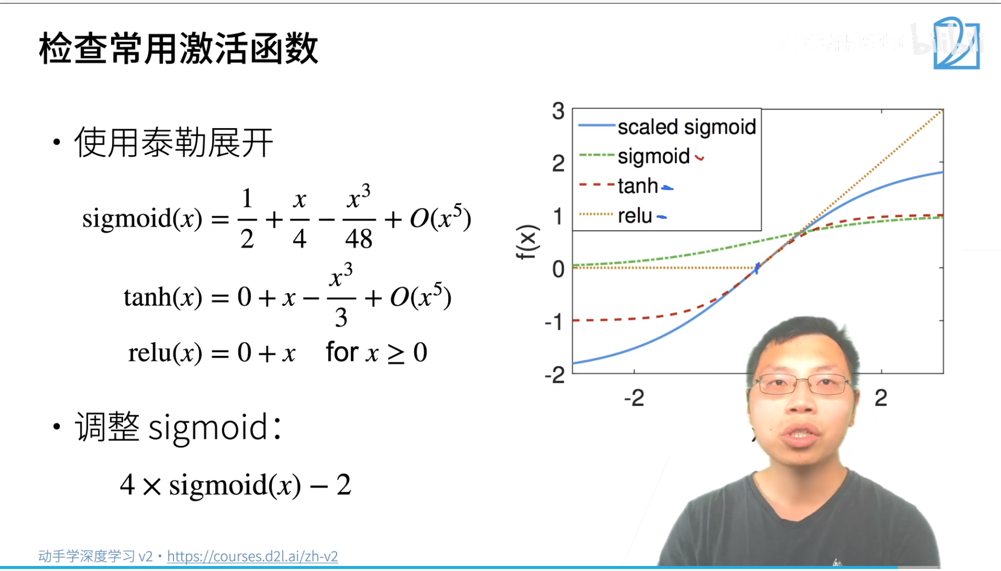
Activation Functions
Sigmoid: 对于一个定义域在$\mathbb{R}$中的输入,sigmoid函数将输入变换为区间(0, 1)上的输出。因此,sigmoid通常称为挤压函数(squashing function):它将范围(-inf, inf)中的任意输入压缩到区间(0, 1)中的某个值:
\[\operatorname{sigmoid}(x) = \frac{1}{1 + \exp(-x)}.\]
sigmoid函数的导数为下面的公式:
\[\frac{d}{dx} \operatorname{sigmoid}(x) = \frac{\exp(-x)}{(1 + \exp(-x))^2} = \operatorname{sigmoid}(x)\left(1-\operatorname{sigmoid}(x)\right).\]
Tanh: Like the sigmoid function, the tanh (hyperbolic tangent) function also squashes its inputs, transforming them into elements on the interval between -1 and 1:
\[\operatorname{tanh}(x) = \frac{1 - \exp(-2x)}{1 + \exp(-2x)} = \frac{exp(x) - \exp(-x)}{exp(x) + \exp(-x)}.\]
函数商的求导法: \(\frac{f(x)}{g(x)} = \frac{f'(x)g(x)-f(x)g'(x)}{g(x)^2}\)
tanh函数的导数是:
\[\frac{d}{dx} \operatorname{tanh}(x) = 1 - \operatorname{tanh}^2(x).\]
Relu(rectified linear unit (ReLU)): [ReLU提供了一种非常简单的非线性变换]。 给定元素$x$,ReLU函数被定义为该元素与$0$的最大值:
\[\operatorname{ReLU}(x) = \max(x, 0).\]
def relu(X):
    a = torch.zeros_like(X)
    return torch.max(X, a)
使用ReLU的原因是,它求导表现得特别好:要么让参数消失,要么让参数通过。这使得优化表现得更好,并且ReLU减轻了困扰以往神经网络的梯度消失问题。
注意,ReLU函数有许多变体,包括参数化ReLU(Parameterized ReLU,pReLU)函数 He. Zhang. Ren.ea.2015 。该变体为ReLU添加了一个线性项,因此即使参数是负的,某些信息仍然可以通过:

mlp = nn.Sequential(nn.Flatten(), nn.Linear(784, 256), nn.ReLU(),
                    nn.Linear(256, 10))
不能将神经网络网络的权重初始化为相同值,如果是 Relu 此时无法通过SGD更新除最后一层bias外的参数进行学习。但是其他激活函数仍然可以更新 {:.warning}
Model Selection, Underfitting, and Overfitting [11]
Weight Decay
通过限制参数取值范围来控制模型容量 在训练参数化机器学习模型时,权重衰减(通常称为$L_2$正则化)是最广泛使用的正则化的技术之一。 实际上,我们通过正则化常数$\lambda$来描述这种权衡,这是一个非负超参数,我们使用验证数据拟合:
\[L(\mathbf{w}, b) + \frac{\lambda}{2} \|\mathbf{w}\|^2,\]对于$\lambda = 0$,我们恢复了原来的损失函数。对于$\lambda > 0$,我们限制$| \mathbf{w} |$的大小。我们仍然除以$2$ 当我们取一个二次函数的导数时,$2$和$1/2$会抵消,以确保更新表达式看起来既漂亮又简单。聪明的读者可能会想知道为什么我们使用平方范数而不是标准范数(即欧几里得距离)。我们这样做是为了便于计算。通过平方$L_2$范数,我们去掉平方根,留下权重向量每个分量的平方和。这使得惩罚的导数很容易计算:导数的和等于和的导数。 使用$L_2$范数,而不是$L_1$范数。事实上,这些选择在整个统计领域中都是有效的和受欢迎的。$L_2$正则化线性模型构成经典的岭回归(ridge regression)算法,$L_1$正则化线性回归是统计学中类似的基本模型,通常被称为套索回归(lasso regression)。
使用$L_2$范数的一个原因是它对权重向量的大分量施加了巨大的惩罚。这使得我们的学习算法偏向于在大量特征上均匀分布权重的模型。在实践中,这可能使它们对单个变量中的观测误差更为鲁棒。相比之下,$L_1$惩罚会导致模型将其他权重清除为零而将权重集中在一小部分特征上。这称为特征选择(feature selection),这可能是其他场景下需要的。较小的$\lambda$值对应较少约束的$\mathbf{w}$,而较大的$\lambda$值对$\mathbf{w}$的约束更大。
def l2_penalty(w):
    return torch.sum(w.pow(2)) / 2
 l = loss(net(X), y) + lambd * l2_penalty(w)

# The bias parameter has not decayed
    trainer = torch.optim.SGD([{
        "params": net[0].weight,
        'weight_decay': wd}, {
            "params": net[0].bias}], lr=lr)
Dropout
在标准dropout正则化中,通过按保留(未丢弃)的节点的分数进行归一化来消除每一层的偏差。换言之,每个中间激活值$h$以丢弃概率$p$由随机变量$h’$替换,如下所示:
\[\begin{aligned} h' = \begin{cases} 0 & \text{ 概率为 } p \\ \frac{h}{1-p} & \text{ 其他情况} \end{cases} \end{aligned}\]根据设计,期望值保持不变,即$E[h’] = h$。
def dropout_layer(X, dropout):
    assert 0 <= dropout <= 1
    # In this case, all elements are dropped out
    if dropout == 1:
        return torch.zeros_like(X)
    # In this case, all elements are kept
    if dropout == 0:
        return X
    mask = (torch.rand(X.shape) > dropout).float()
    # mask = (torch.Tensor(X.shape).uniform_(0, 1) > dropout).float()
    return mask * X / (1.0 - dropout)

class Net(nn.Module):
    def __init__(self, num_inputs, num_outputs, num_hiddens1, num_hiddens2,
                 is_training = True):
        super(Net, self).__init__()
        self.num_inputs = num_inputs
        self.training = is_training
        self.lin1 = nn.Linear(num_inputs, num_hiddens1)
        self.lin2 = nn.Linear(num_hiddens1, num_hiddens2)
        self.lin3 = nn.Linear(num_hiddens2, num_outputs)
        self.relu = nn.ReLU()

    def forward(self, X):
        H1 = self.relu(self.lin1(X.reshape((-1, self.num_inputs))))
        # 只有在训练模型时才使用dropout
        if self.training == True:
            # 在第一个全连接层之后添加一个dropout层
            H1 = dropout_layer(H1, dropout1)
        H2 = self.relu(self.lin2(H1))
        if self.training == True:
            # 在第二个全连接层之后添加一个dropout层
            H2 = dropout_layer(H2, dropout2)
        out = self.lin3(H2)
        return out

net = nn.Sequential(nn.Flatten(),
        nn.Linear(784, 256),
        nn.ReLU(),
        # 在第一个全连接层之后添加一个dropout层
        nn.Dropout(dropout1),
        nn.Linear(256, 256),
        nn.ReLU(),
        # 在第二个全连接层之后添加一个dropout层
        nn.Dropout(dropout2),
        nn.Linear(256, 10))
梯度消失和梯度爆炸
考虑一个具有$L$层、输入$\mathbf{x}$和输出$\mathbf{o}$的深层网络。每一层$l$由变换$f_l$定义,该变换的参数为权重$\mathbf{W}^{(l)}$,其隐藏变量是$\mathbf{h}^{(l)}$(令 $\mathbf{h}^{(0)} = \mathbf{x}$)。我们的网络可以表示为:
\[\mathbf{h}^{(l)} = f_l (\mathbf{h}^{(l-1)}) \text{ 因此 } \mathbf{o} = f_L \circ \ldots \circ f_1(\mathbf{x}).\]如果所有隐藏变量和输入都是向量,我们可以将$\mathbf{o}$关于任何一组参数$\mathbf{W}^{(l)}$的梯度写为下式:
\[\partial_{\mathbf{W}^{(l)}} \mathbf{o} = \underbrace{\partial_{\mathbf{h}^{(L-1)}} \mathbf{h}^{(L)}}_{ \mathbf{M}^{(L)} \stackrel{\mathrm{def}}{=}} \cdot \ldots \cdot \underbrace{\partial_{\mathbf{h}^{(l)}} \mathbf{h}^{(l+1)}}_{ \mathbf{M}^{(l+1)} \stackrel{\mathrm{def}}{=}} \underbrace{\partial_{\mathbf{W}^{(l)}} \mathbf{h}^{(l)}}_{ \mathbf{v}^{(l)} \stackrel{\mathrm{def}}{=}}.\]换言之,该梯度是$L-l$个矩阵$\mathbf{M}^{(L)} \cdot \ldots \cdot \mathbf{M}^{(l+1)}$与梯度向量 $\mathbf{v}^{(l)}$的乘积。因此,我们容易受到数值下溢问题的影响,当将太多的概率乘在一起时,这些问题经常会出现。在处理概率时,一个常见的技巧是切换到对数空间,即将数值表示的压力从尾数转移到指数。不幸的是,我们上面的问题更为严重:最初,矩阵 $\mathbf{M}^{(l)}$ 可能具有各种各样的特征值。他们可能很小,也可能很大,他们的乘积可能非常大,也可能非常小。
不稳定梯度带来的风险不止在于数值表示。不稳定梯度也威胁到我们优化算法的稳定性。我们可能面临一些问题。 要么是 梯度爆炸(gradient exploding)问题:参数更新过大(lr太大),破坏了模型的稳定收敛; 要么是 梯度消失(gradient vanishing)问题:参数更新过小(lr太小),在每次更新时几乎不会移动,导致无法学习。
让训练更加稳定:
- Goal: 让梯度在合理的范围之内,例如[1e-6, 1e3]
- 将乘法变加法: ResNet,LSTM
- 归一化: 梯度归一化,梯度裁剪
- 合理的权重初始化和激活函数
Xavier初始化
让我们看看某些没有非线性的全连接层输出(例如,隐藏变量)$o_{i}$的尺度分布。 对于该层$n_\mathrm{in}$输入$x_j$及其相关权重$w_{ij}$,输出由下式给出
\[o_{i} = \sum_{j=1}^{n_\mathrm{in}} w_{ij} x_j.\]权重$w_{ij}$都是从同一分布中独立抽取的。此外,让我们假设该分布具有零均值和方差$\sigma^2$。请注意,这并不意味着分布必须是高斯的,只是均值和方差需要存在。现在,让我们假设层$x_j$的输入也具有零均值和方差$\gamma^2$,并且它们独立于$w_{ij}$并且彼此独立。在这种情况下,我们可以按如下方式计算$o_i$的平均值和方差:
\[\begin{aligned} E[o_i] & = \sum_{j=1}^{n_\mathrm{in}} E[w_{ij} x_j] \\&= \sum_{j=1}^{n_\mathrm{in}} E[w_{ij}] E[x_j] \\&= 0, \\ \mathrm{Var}[o_i] & = E[o_i^2] - (E[o_i])^2 \\ & = \sum_{j=1}^{n_\mathrm{in}} E[w^2_{ij} x^2_j] - 0 \\ & = \sum_{j=1}^{n_\mathrm{in}} E[w^2_{ij}] E[x^2_j] \\ & = n_\mathrm{in} \sigma^2 \gamma^2. \end{aligned}\]保持方差不变的一种方法是设置$n_\mathrm{in} \sigma^2 = 1$。现在考虑反向传播过程,我们面临着类似的问题,尽管梯度是从更靠近输出的层传播的。使用与正向传播相同的推理,我们可以看到,除非$n_\mathrm{out} \sigma^2 = 1$,否则梯度的方差可能会增大,其中$n_\mathrm{out}$是该层的输出的数量。这使我们进退两难:我们不可能同时满足这两个条件。相反,我们只需满足:
\[\begin{aligned} \frac{1}{2} (n_\mathrm{in} + n_\mathrm{out}) \sigma^2 = 1 \text{ 或等价于 } \sigma = \sqrt{\frac{2}{n_\mathrm{in} + n_\mathrm{out}}}. \end{aligned}\]这就是现在标准且实用的Xavier初始化的基础,它以其提出者 Glorot. Bengio.2010 第一作者的名字命名。通常,Xavier初始化从均值为零,方差$\sigma^2 = \frac{2}{n_\mathrm{in} + n_\mathrm{out}}$的高斯分布中采样权重。我们也可以利用Xavier的直觉来选择从均匀分布中抽取权重时的方差。注意均匀分布$U(-a, a)$的方差为$\frac{a^2}{3}$。将$\frac{a^2}{3}$代入到$\sigma^2$的条件中,将得到初始化的建议:
尽管上述数学推理中,不存在非线性的假设在神经网络中很容易被违反,但Xavier初始化方法在实践中被证明是有效的。
def xavier(m):
    if type(m) == nn.Linear:
        nn.init.xavier_uniform_(m.weight)
K-flod
def get_k_fold_data(k, i, X, y):
    assert k > 1
    fold_size = X.shape[0] // k
    X_train, y_train = None, None
    for j in range(k):
        idx = slice(j * fold_size, (j + 1) * fold_size)
        X_part, y_part = X[idx, :], y[idx]
        if j == i:
            X_valid, y_valid = X_part, y_part
        elif X_train is None:
            X_train, y_train = X_part, y_part
        else:
            X_train = torch.cat([X_train, X_part], 0)
            y_train = torch.cat([y_train, y_part], 0)
    return X_train, y_train, X_valid, y_valid

def k_fold(k, X_train, y_train, num_epochs, learning_rate, weight_decay,
           batch_size):
    train_l_sum, valid_l_sum = 0, 0
    for i in range(k):
        data = get_k_fold_data(k, i, X_train, y_train)
        net = get_net()
        train_ls, valid_ls = train(net, *data, num_epochs, learning_rate,
                                   weight_decay, batch_size)
        train_l_sum += train_ls[-1]
        valid_l_sum += valid_ls[-1]
        if i == 0:
            d2l.plot(list(range(1, num_epochs + 1)), [train_ls, valid_ls],
                     xlabel='epoch', ylabel='rmse', xlim=[1, num_epochs],
                     legend=['train', 'valid'], yscale='log')
        print(f'fold {i + 1}, train log rmse {float(train_ls[-1]):f}, '
              f'valid log rmse {float(valid_ls[-1]):f}')
    return train_l_sum / k, valid_l_sum / k